
Emergence of unique hues from sparse coding of color in natural images
Alexander Belsten, E. Paxon Frady, and Bruno A. Olshausen
Published July 14th, 2026 in JOSA A. https://doi.org/10.1364/JOSAA.598897
In this blog post, I explain our recent findings on color vision for a general audience. The paper makes two main contributions. First, we show that the distribution of colors in natural images is highly non-random. Second, we show that when a statistical model called sparse coding is fit to this distribution, it converges to a specific set of basis vectors in color space that are also considered ‘unique’ by humans.
I will keep the specific details of color to a minimum, as color can get quite technical. Of course, the details are in the paper. There are also many excellent resources on color vision, including Brian Wandell’s Foundations of Vision.
Sparse coding also comes with its own jargon and complexities. Here, I hope to shed some of that, as applying this method to a low-dimensional color space lends itself to an intuitive geometric understanding of what this model is doing.
Let’s begin with some history.
What are the unique hues?
Why do red, green, blue, and yellow seem more “pure” than other colors?
For example, while the color purple might naturally be described as a combination of red and blue, it seems somewhat less intuitive to think of red as a combination of orange and purple, even though a mixture of those colors would produce red just as well as red + blue produce purple. In other words, we tend to think of red as just red, not as a mixture. This same unique property holds for green, blue, and yellow: each appears perceptually pure rather than as a mixture of neighboring hues.
This phenomenon was first described and extensively documented in the late 19th century by the German physiologist Ewald Hering, who dubbed these unique colors the Urfarben. He proposed that they serve as a perceptual basis for describing all other colors, and moreover, that certain pairs of these colors – red/green and blue/yellow – appear opposites in that they are never used simultaneously to describe any color. Just as one would never say you are traveling in an east-west or north-south direction, it would be just as nonsensical to describe a color as appearing reddish-green or bluish-yellow.
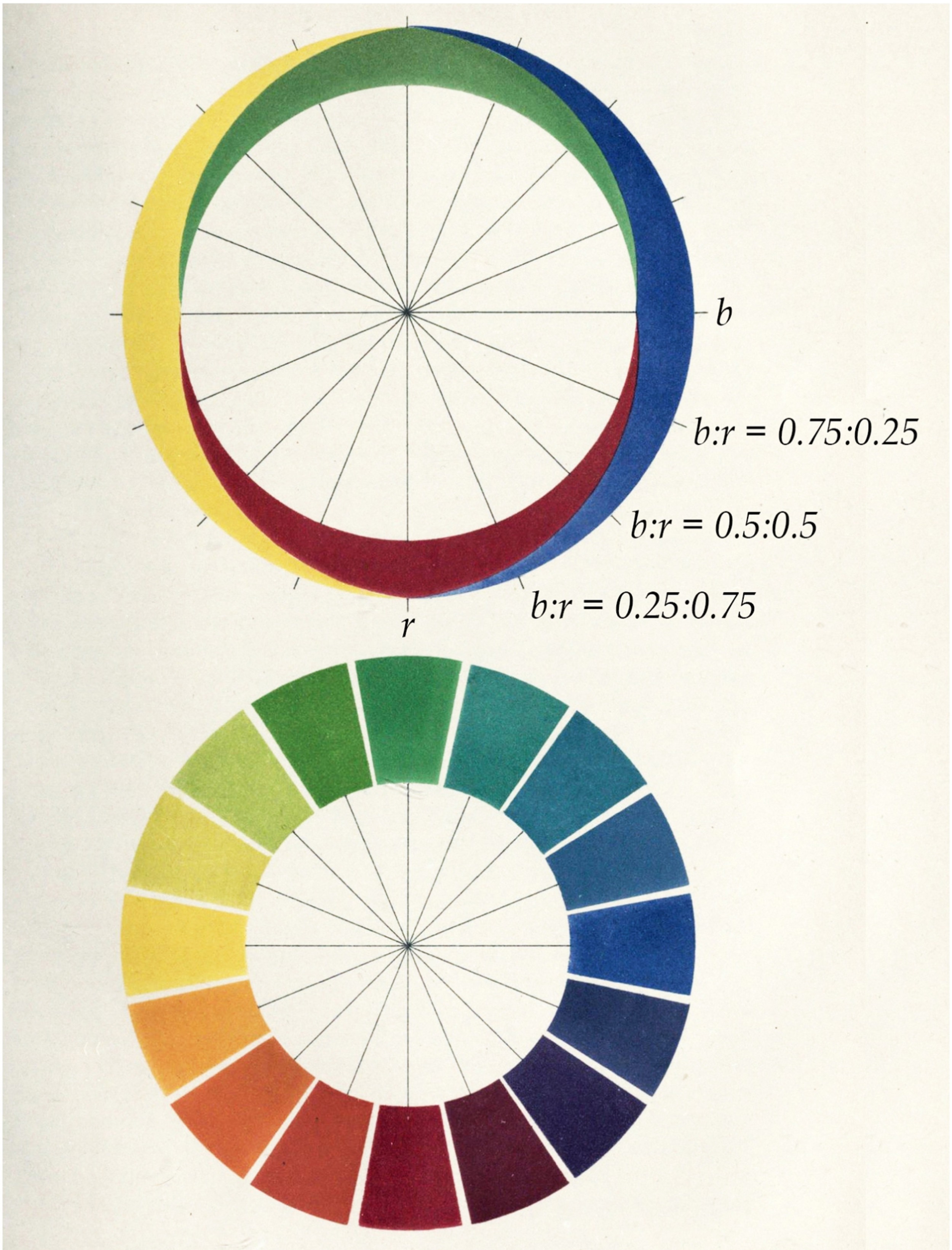
More than a century later, the unique hues and their opponent nature still serve as the accepted basis for describing color appearance, yet their special status remains a mystery. No known property of light, the cone photoreceptors in the eye, or neural representations in the brain can explain why these four hues, rather than some other set, should occupy this privileged position (Conway et al., 2023; Mollon & Jordan, 1997).
Our study suggests that the answer to the perceptual mystery lies in the distribution of colors present in the natural world. By simulating how each of the three types of human cone photoreceptors respond to hundreds of millions of points sampled from natural scenes, obtained from publicly available datasets of calibrated color images acquired from diverse locations around the world, we find that the distribution of colors is non-random. Most pixels are relatively achromatic (colorless), while highly saturated colors are rarer. But those rare colors are not spread equally in every direction: some occur with greater saturation consistently more often than others. To characterize this structure in the distribution, we fit a model to the data that finds a set of basis vectors to optimally span color space such that a weighted sum of them can describe any color using a minimal total sum of weights on average. When the model is given four basis vectors to describe hue, they converge on the unique hues – red, green, blue, and yellow. Moreover, the opposing nature of red-green and blue-yellow also emerges from the model since these vectors are never used in combination to describe any other color, exactly as proposed by Hering more than a century ago. Together, these findings shed new light on the distribution of color in the natural environment and provide a linking principle between this structure and the phenomenology of color appearance.
A color basis
Hering was, in effect, describing the unique hues as a natural basis for reasoning about colors. This idea can be formalized using the mathematical concept of a basis: a collection of elementary directions that can be combined to represent other points in a space.
For example, a hue can be represented as a point in color space. Just as there are infinitely many points in a real-valued space, there are infinitely many hues. But any given point $\mathbf{x}$ can be described through a linear combination of a finite set of $m$ basis vectors $\mathbf{a}_i$ weighted by coefficients $s_i$,
\[\mathbf{x} = \sum_{i=1}^m \mathbf{a}_i\, s_i \,,\]as long as $m$ is greater than or equal to the dimensionality of the space. The basis vectors specify the available elementary color directions, while the coefficients specify how much of each direction is used to represent a particular color.
To keep the geometry simple, let’s assume that changes in luminance have been accounted for, so only variation in hue and saturation needs to be considered. In the paper, we consider a full three-dimensional color space that includes luminance, but we can make the major points by just considering the chromatic plane, making color points $\mathbf{x}$ and basis vectors $\mathbf{a}_i$ two-dimensional. Within this color space, a color point’s saturation is given by its distance from the origin and its hue is given by its angle.
A nominal arrangement that spans this two-dimensional space is a set of three basis vectors separated by 120${}^\circ$, forming a so-called `Mercedes-Benz frame’. Such a basis is shown in Figure 2.
Given this basis, how should we choose the coefficients to represent a particular color? We use a constructive representation, meaning that the coefficients must be nonnegative: colors are represented by adding basis directions rather than subtracting them. We also favor sparse reconstructions, which favors using only a small number of basis vectors out the larger dictionary to reconstruct the data point.
The process of finding these nonnegative, sparse coefficients is called sparse inference (or inference for short). Sparse inference jointly adjusts the coefficients until the weighted basis vectors accurately reconstruct the target color while keeping the total coefficient activity small. This process requires a joint optimization because, in general, the basis vectors are not orthogonal so changing one coefficient changes the residual that the others must explain. Thus, an iterative algorithm that repeatedly adjusts the coefficients until an accurate reconstruction is found is needed.
The animation in Figure 2 shows the process of inference for three colors using the Mercedes-Benz frame:
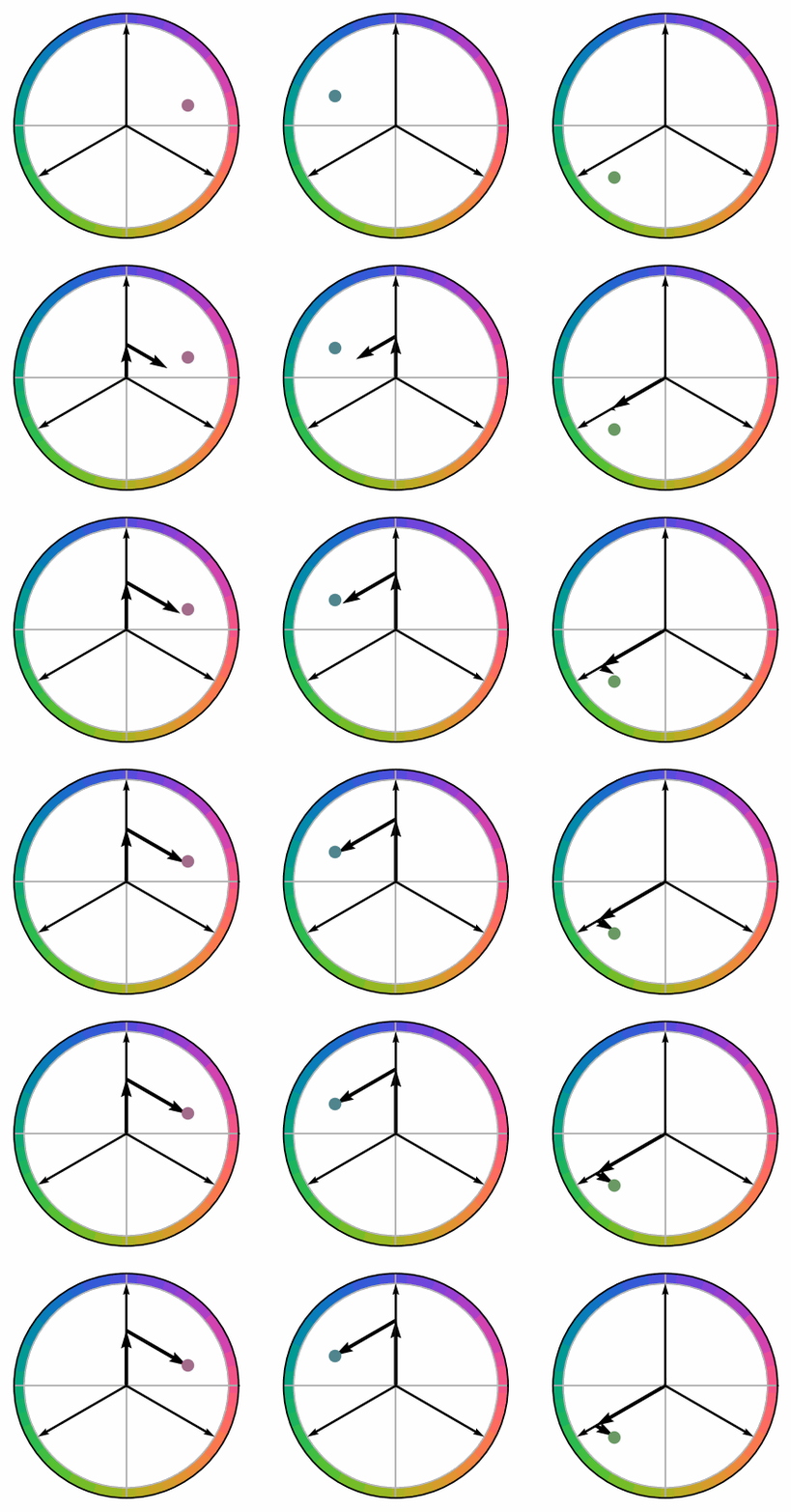
Each basis vector is rescaled by its corresponding coefficient, and geometrically placing the scaled vectors end to end shows how their sum reaches the target color. Because the basis vectors have unit length, the sum of the coefficients is also the total path length traced by the scaled vectors. In general, more saturated colors will have a longer path length. Sparse inference favors a short path to the target. In this two-dimensional example, at most two basis vectors are necessary to represent any color, and only one is needed when the target lies directly along a basis direction.
With this geometric view, we can see how activating all three vectors would introduce unnecessary backtracking. Since $\mathbf{x}$ is 2-dimensional, the minimum-path representation uses no more than two active coefficients. This is not unique to the Mercedes-Benz frame or even having three basis vectors. Given a basis of size $m>n+1$ that spans an $n$-dimensional space under nonnegative weightings, only $n$ nonzero coefficients are needed to represent a point in that space.
The statistical model we’re describing is called sparse coding. Sparse coding assumes that the data can be represented using sparse coefficients on a collection of basis vectors (Olshausen & Field, 1996). The mathematical details of sparse coding and sparse inference are described below. Readers interested primarily in the main results can skip this box.
Mathematical details: sparse coding inference
While reconstructing a data point from the coefficients is linear, $\mathbf{x} = \sum_i {a}_i\,s_i$, computing the coefficients $s_1,s_2,…,s_m$ given a datapoint $\mathbf{x}$ is nonlinear. For a given $\mathbf{x}$, the $s_i$ are computed by minimizing a sparse coding energy function $E$ subject to a nonnegativity constraint:
\[\begin{align} \min_{\{s_i\}_{i=1}^m} & \quad E = \frac{1}{2}\Big\lVert\mathbf{x} - \sum_{i=1}^m\mathbf{a}_i{s}_i\Big\rVert_2^2\; +\; \lambda \sum_{i=1}^m s_i \label{eqn:energy} \\ \text{subject to} & \quad s_i \geq 0 \quad\text{for} \ i = 1,2,...,m. \end{align}\]The first term in this energy function says that the coefficients should reconstruct the data point, while the second term imposes a $\ell_1$-sparsity inducing penalty that encourages using only a small number of basis vectors out the larger dictionary ${\mathbf{a}_i}$. The parameter $\lambda$ controls the trade-off between reconstruction quality and sparsity.
Given a set of basis vectors, the above optimization problem can be solved using a nonnegative variant of the locally competitive algorithm (LCA; Rozell et al., 2008). LCA evolves subthreshold variables $u_i$ whose thresholded outputs $s_i$ are the coefficients:
\[\begin{align} \tau \dot{u}_i + u_i &= \mathbf{a}_i^T\mathbf{x} - \sum_{j\neq i}\mathbf{G}_{ij} s_j \\ s_i &= \max(0, u_i-\lambda) = g(u_i), \end{align}\]where $ \mathbf{G}_{ij} = \mathbf{a}_i^T\mathbf{a}_j$. The rectifying nonlinearity $g(\cdot)$ enforces the $\ell_1$-sparsity penalty on the coefficients while imposing an infinite energy barrier at $s_i<0$, satisfying the nonnegativity constraint. Letting the dynamics above settle to an equilibrium yields the nonnegative coefficients that minimize $E$.
We refer to the process of computing the coefficients as inference because it is actually performing maximum-a-posteriori (MAP) Bayesian inference (for details see Olshausen & Field, 1997).
So far, we have fixed the basis to a Mercedes-Benz frame. But this choice is arbitrary: infinitely many other arrangements could also represent every hue. How should we choose among them? One possibility is that the visual system adapts its representation to the colors it repeatedly encounters, favoring basis vectors that efficiently capture the statistical structure of the natural environment. Color perception has long been proposed to reflect such environmental statistics (e.g., Mollon & Jordan, 1997; Shepard, 1992; Skelton et al., 2024). Could this adaptation explain the unique hues?
The distribution of color in natural images is highly non random
To measure the distribution of color in the natural environment, we combined publicly available datasets of calibrated color images acquired from diverse locations around the world. Figure 3 shows a few examples from the dataset.
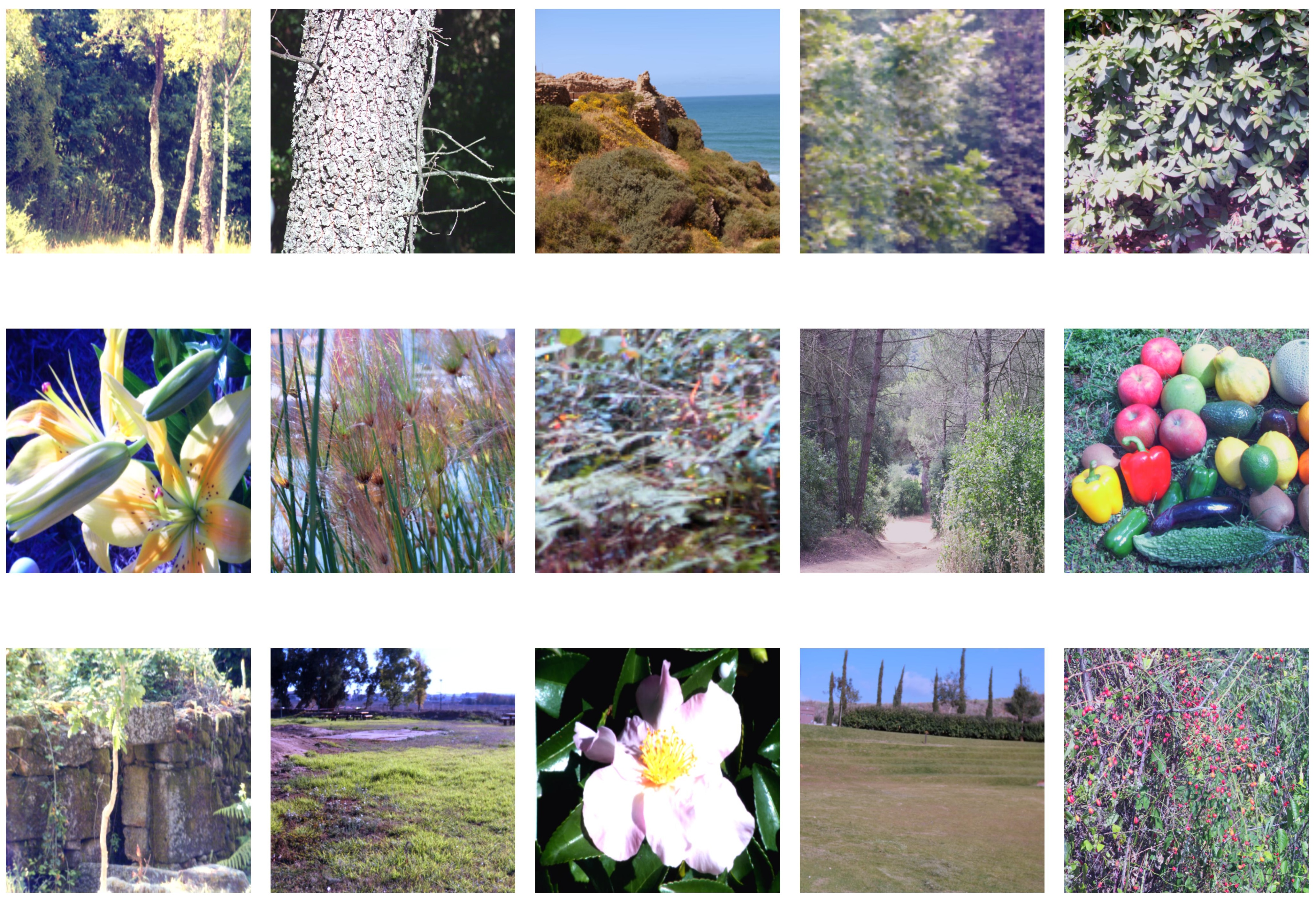
The dataset contains 503 images of flora, forests, landscapes, seascapes, and geological formations, yielding over 225 million pixels for analysis. We excluded scenes containing human-made objects because their colors may reflect human perceptual and design preferences and thus could inherit the very biases in human color perception that we seek to study.
We seek to understand how color is distributed in this dataset. 225 million data points is far too many to put in a scatterplot. Instead, we project the entire three-dimensional distribution of pixels onto the chromatic plane and compute a histogram of the projections. We then summarize this histogram using iso-probability contours, as shown below:
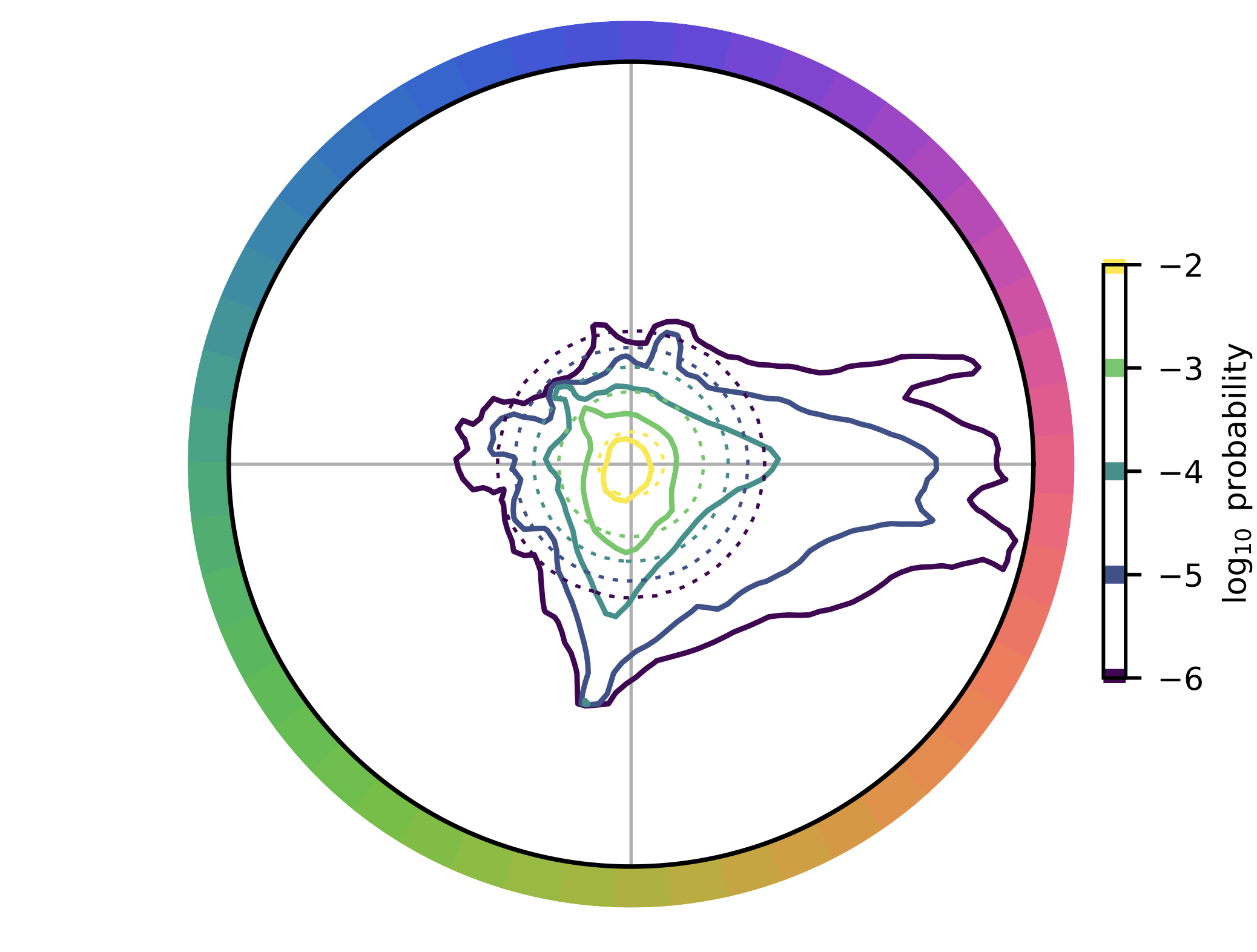
As a reminder, a color’s position in the chromatic plane represents its hue and saturation: hue corresponds to angular direction, while chromatic saturation corresponds to radial distance from the origin.
The largest probability contour is near the origin, meaning that most pixels are relatively achromatic (colorless). Lower probability contours are further from the origin indicating that highly saturated colors are more rare. However, the iso-probability contours are not perfect circles. Instead, they are anisotropic and extend in certain hue directions — most notably toward red. Colors in natural scenes are not distributed equally across hue directions.
The distribution is also asymmetric: hue directions that are opposite to one another in the space do not necessarily have the same probability profile. We find that this structure is generally persistent across heterogeneous datasets.
In the plot above, we have scaled the chromatic axes such that the data have unit variance in every direction (Ruderman et al., 1998). This makes an isotropic Gaussian a reference for what distribution of colors would be truly random. The contours of this distribution are overlaid in dashed lines. Importantly, if the distribution were Gaussian, the solid contours would follow the dashed contours exactly, but this is not the case. Comparing the isoprobability contours of the natural image distribution to those of the Gaussian reveals pronounced asymmetries and substantial deviations from Gaussianity. Colors in natural scenes have a non random distribution. Specifically, the distribution contains heavy-tailed structure as matched iso-probability contours of the true distribution extend further from the origin than that of the Gaussian.
These heavy tails and asymmetries are examples of higher-order statistical structure which can not be characterized using pair-wise correlations (Simoncelli & Olshausen, 2001). We believe that this higher-order structure has implications for how the brain represents color.
The idea that the brain is adapted to higher-order statistics in sensory input is not a new one. For example, David Field (1987) showed correspondence between the higher-order statistical structure of natural image patches and orientation-selective spatial receptive properties of simple-cells in visual cortex (which eventually led to the development of the sparse coding model). There is also correspondence between auditory nerve fiber tuning properties and the statistical structure of environmental sounds and vocalizations (Lewicki, 2002).
Adapting the basis to model non-Gaussian structure
Given the non-Gaussian structure of color in natural images, some basis vector directions will be preferable under the sparsity assumption. Therefore, we now turn to learning: adapting the basis vectors themselves to the distribution of colors in natural scenes.
When the basis is adapted to the structure in the data, the puzzle the model is solving is how to place these vectors in the space such that there is a maximally sparse nonnegative code produced in the coefficients when averaged over the entire dataset. Doing so favors learning basis vectors that align with the directions in the data which occur rarely but with high magnitude, i.e., the heavy-tailed directions. Thus, the model learns a concise and efficient way to represent color and the higher-order statistical structure of natural colors.
The mathematical details of the learning rule are given below. This box can be skipped without disrupting the main results.
Mathematical details: learning the sparse coding basis vectors
The basis vectors $\mathbf{a}_i$ are adapted to the structure of the data by stochastic gradient descent on $E$, using the inferred coefficients $s_i$ for each data sample $\mathbf{x}$. This yields the following learning rule:
\[\begin{align} \Delta \mathbf{a}_i = \eta \left[ \mathbf{x} - \sum_{j=1}^m \mathbf{a}_j s_j \right] s_i. \end{align}\]The update rate $\eta$ is set so that the energy decreases continuously until convergence. After each update, the basis vectors are normalized to have unit norm: $\lVert\mathbf{a}_i\rVert_2 =1 \text{ for all } i$.
The animation below shows this learning process for a model with three basis vectors. Each panel begins from a different random initialization.
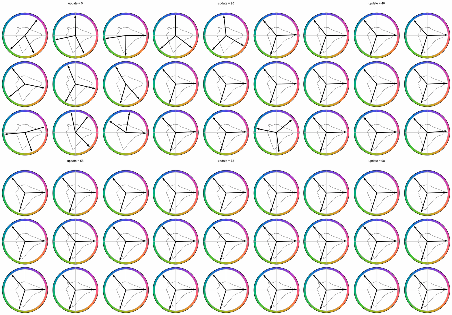
Despite their different starting points, the models converge to the same general arrangement: the three basis vectors that correspond to blue, red, and green-yellow. This placement is expected, as the data exhibits a heavy-tailed extension in these directions, as indicated by the iso-probability contour overlayed on each subplot.
But three vectors are only one possible choice. What happens when the model is given a fourth? Learning four basis vectors is shown in the animation below.
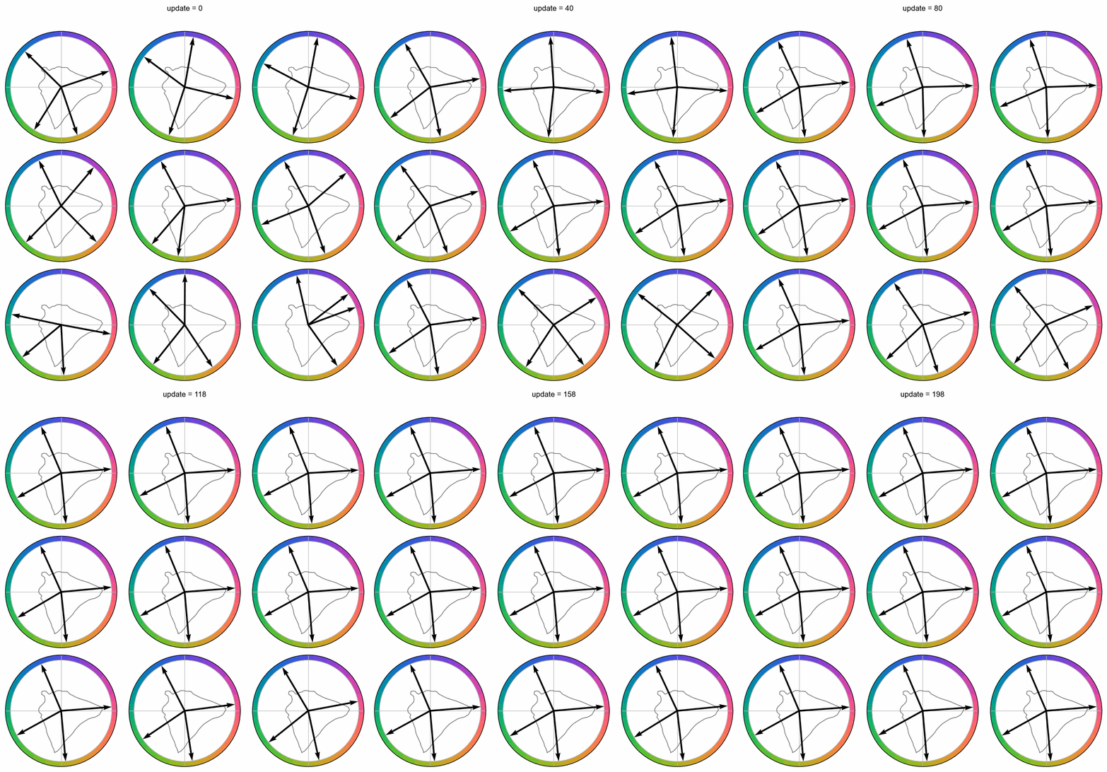
Compared with the three-vector solution, the red vector remains relatively stable. Adding a fourth vector splits the broad blue–green region: a new vector settles near green, while the neighboring vectors shift toward blue and yellow. The resulting arrangement aligns approximately with red, green, blue, and yellow.
Human measurements suggest that the unique hues are not orthogonal to one another, and thus opponent pairs such as red–green and blue–yellow are not diametrically opposite in a geometric color plane. The learned basis reproduces these qualitative attributes.
Emergence of color opponency
What mathematical principles could reproduce such an opponent organization?
Recall that sparse inference will only use at most two basis vectors at a time to represent a point in the two-dimensional color space. We find that this naturally gives rise to mutual exclusivity between basis vector coefficients that represent phenomenologically opposing colors (red/green and blue/yellow). Figure 7 demonstrates this. The left side of the plot shows how the point is reconstructed by combining the weighted basis vectors end-to-end, and the right side shows the coefficient magnitudes.
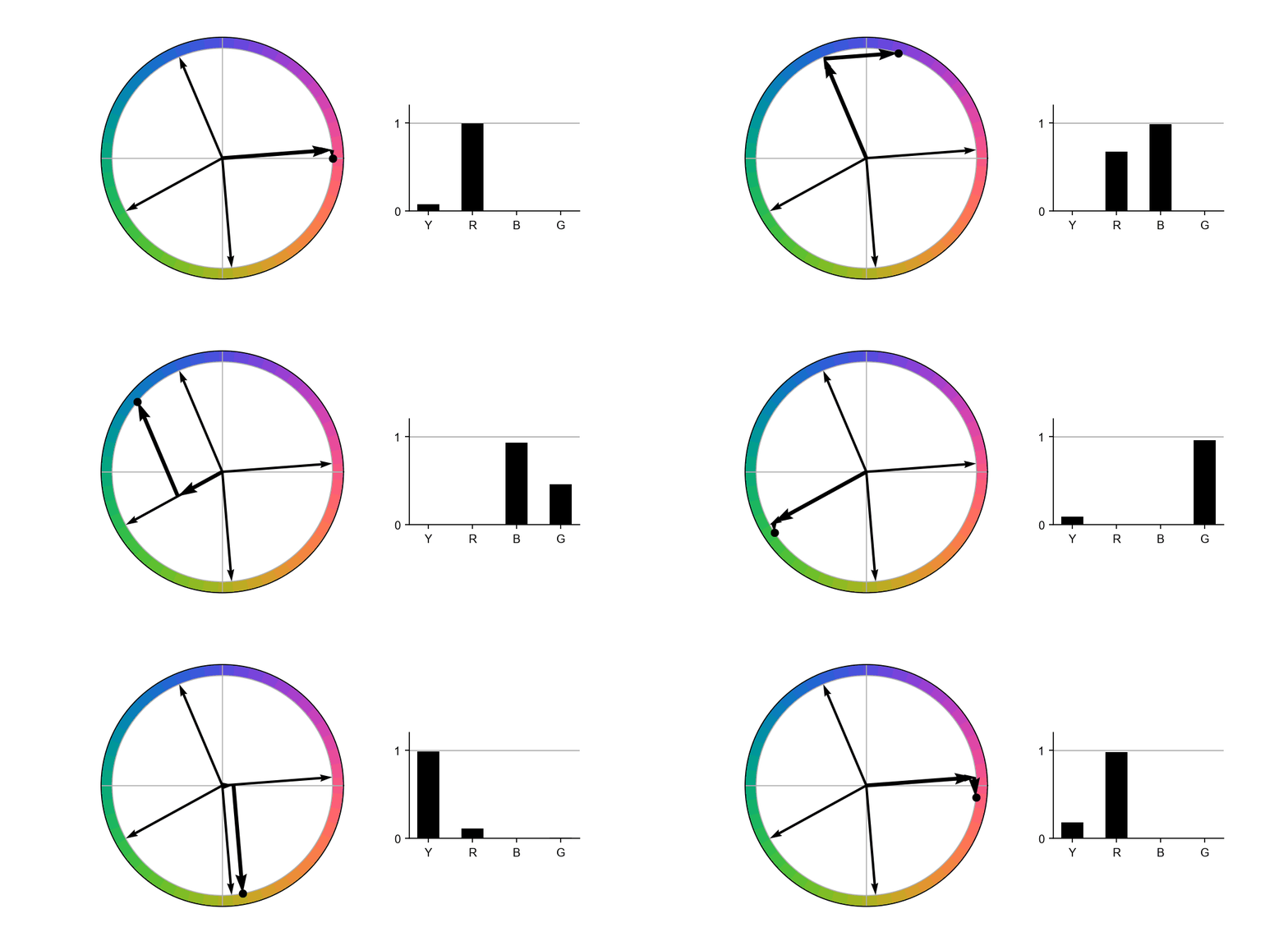
As the target moves around the hue circle, neighboring basis vectors activate together to represent intermediate hues. By contrast, red and green are never coactive, nor are blue and yellow. This opposition was not imposed on the model but emerges from sparse inference.
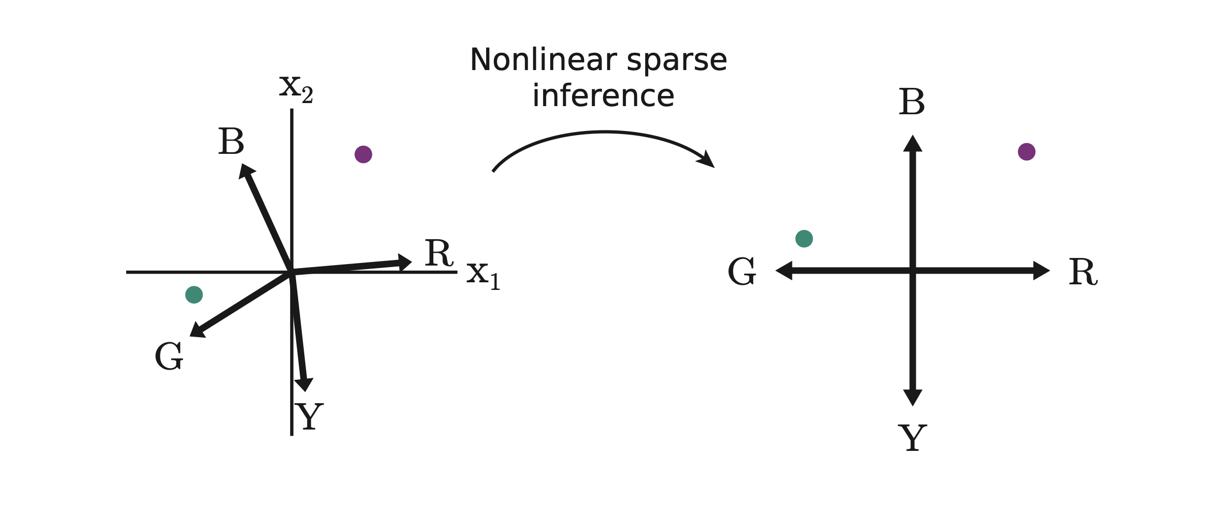
Although the learned basis vectors are not geometrically opposite in the original color space, their inferred coefficients can be reorganized into two signed opponent axes as shown in Figure 8. Red and green occupy opposite ends of one axis, while blue and yellow occupy opposite ends of the other. This two-dimensional opponent space captures the phenomenological organization of color experience.
You might be wondering: why favor four basis vectors over three? Both models can represent any point in the color plane and thus form a complete code. You might argue that the three basis vector model is better aligned with the heavy-tails in the data. A distinction between them lies in the structure of the resulting sparse code. In the three-vector model, the coefficients exhibit a three-way dependency: when two are active, the third is silent. In the four-vector model, this dependency separates into two mutually exclusive pairs, red versus green and blue versus yellow, which can be collapsed into two sets of opposing axes. This points to a trade-off between being perfectly aligned with the data vs. producing a parsimonious distributed code.
Conclusion
The two main contributions of this paper are (1) the finding of strongly non-Gaussian structure of color in a large database of natural images, and (2) showing that a constructive linear generative model adapted to this data aligns with the unique hues. Sparse coding inference introduces mutual exclusivity between coefficients and yields a color representation that mirrors the phenomenology of color perception. It is remarkable that not only unique hues but also the structure of their interactions arises from fitting a single linear generative model, with few other assumptions, to the data.
References
Conway, B. R., Malik-Moraleda, S., & Gibson, E. (2023). Color appearance and the end of Hering’s Opponent-Colors Theory. Trends in Cognitive Sciences, 27(9), 791-804.
Field, D. J. (1987). Relations between the statistics of natural images and the response properties of cortical cells. Journal of the Optical Society of America A, 4(12), 2379-2394.
Lewicki, M. S. (2002). Efficient coding of natural sounds. Nature neuroscience, 5(4), 356-363.
Mollon, J. D., & Jordan, G. (1997). On the nature of unique hues. John Dalton’s colour vision legacy, 381-392.
Olshausen, B. A., & Field, D. J. (1996). Emergence of simple-cell receptive field properties by learning a sparse code for natural images. Nature, 381(6583), 607-609.
Olshausen, B. A., & Field, D. J. (1997). Sparse coding with an overcomplete basis set: A strategy employed by V1?. Vision research, 37(23), 3311-3325.
Rozell, C. J., Johnson, D. H., Baraniuk, R. G., & Olshausen, B. A. (2008). Sparse coding via thresholding and local competition in neural circuits. Neural computation, 20(10), 2526-2563.
Ruderman, D. L., Cronin, T. W., & Chiao, C. C. (1998). Statistics of cone responses to natural images: implications for visual coding. Journal of the Optical Society of America A, 15(8), 2036-2045.
Shepard, R. N. (1992). The perceptual organization of colors: an adaptation to regularities of the terrestrial world?.
Simoncelli, E. P., & Olshausen, B. A. (2001). Natural image statistics and neural representation. Annual review of neuroscience, 24(1), 1193-1216.
Skelton, A. E., Maule, J., Floyd, S., Wozniak, B., Majid, A., Bosten, J. M., & Franklin, A. (2024). Effects of visual diet on colour discrimination and preference. Proceedings of the Royal Society B: Biological Sciences, 291(2031), 20240909.